Verarbeitung von Sentinel-5P-Daten zur Luftverschmutzung mit Jupyter Notebook auf CODE-DE

Voraussetzungen

Nr. 1 Konto

Sie brauchen ein CODE-DE Konto mit Zugriff auf die Horizon-Schnittstelle: https://cloud.fra1-1.cloudferro.com/auth/login/?next=/.

Nr. 2 Installation von Jupyter Notebook

Der Code in diesem Artikel läuft auf Jupyter Notebook und Sie können es auf der Plattform Ihrer Wahl installieren, indem Sie der offiziellen Jupyter Notebook -Installationsseite folgen.

Eine besondere Art der Installation (nicht erforderlich, um diesem Artikel zu folgen) ist die Installation auf einem Kubernetes-Cluster, die hier beschrieben ist:

/kubernetes/Installing-JupyterHub-on-Magnum-Kubernetes-cluster-in-CODE-DE-cloud.

TEIL #1 - Daten herunterladen und vorbereiten

In diesem Handbuch wird beschrieben, wie man Sentinel-5P-Daten mit Hilfe von HARP und der CREODIAS-Plattform verarbeitet und für die weitere Analyse vorbereitet.

In diesem Notizbuch lernen Sie, wie man:

eine Abfrage über https://explore.creodias.eu/ erstellt

Daten aus dem CREODIAS-Repository von eodata hochladen

ausgewählte Sentinel-5P-Bilder (netCDF) lesen

Sentinel-5P-Bilder (troposphärische NO2-Säule - NO2 TVCD) mit HARP verarbeiten

Erstellen eines Produkt, das den monatlichen Durchschnitt der NO2 TVCD (netCDF) darstellt

Darstellung der Ergebnisse

Zu verwendende Datensätze:

Sentinel-5P (product L2__NO2___) - 01.03.2023 - 31.03.2023; beschränkt auf Polen

Bezirke in Polen https://www.geoportal.gov.pl/dane/panstwowy-rejestr-granic

HARP https://atmospherictoolbox.org/harp/

Bibliotheken importieren

import harp
import numpy as np
import matplotlib.pyplot as plt
import cartopy.crs as ccrs
import cartopy.io.img_tiles as cimgt
from cmcrameri import cm
import json, requests, os

Hochladen von Daten mit einer vom Data Explorer generierten Abfrage

Zusätzlich können Sie den Zeitpunkt der Analyse festlegen:

start	erster Tag des analysierten Zeitraums
end	letzter Tag des analysierten Zeitraums

start = str("2023-03-01") #first day of the analysed period
end = str("2023-03-31")   #last day of the analysed period

#querry generated by Data Explorer
url = f"https://datahub.creodias.eu/odata/v1/Products?$filter=((ContentDate/Start ge {start}T00:00:00.000Z and ContentDate/Start le {end}T23:59:59.999Z) and (Online eq true) and (OData.CSC.Intersects(Footprint=geography'SRID=4326;POLYGON ((13.44866 55.702105, 24.616418 55.287061, 24.505406 48.582106, 13.359851 49.556626, 13.44866 55.702105))')) and (((((((Attributes/OData.CSC.StringAttribute/any(i0:i0/Name eq 'productType' and i0/Value eq 'L2__NO2___')))) and (((Attributes/OData.CSC.StringAttribute/any(i0:i0/Name eq 'processingMode' and i0/Value eq 'OFFL')))) and (Collection/Name eq 'SENTINEL-5P'))))))&$expand=Attributes&$top=1000"

#take a look on result url
"https://datahub.creodias.eu/odata/v1/Products?$filter=((ContentDate/Start ge 2023-03-01T00:00:00.000Z and ContentDate/Start le 2023-03-31T23:59:59.999Z) and (Online eq true) and (OData.CSC.Intersects(Footprint=geography'SRID=4326;POLYGON ((13.44866 55.702105, 24.616418 55.287061, 24.505406 48.582106, 13.359851 49.556626, 13.44866 55.702105))')) and (((((((Attributes/OData.CSC.StringAttribute/any(i0:i0/Name eq 'productType' and i0/Value eq 'L2__NO2___')))) and (((Attributes/OData.CSC.StringAttribute/any(i0:i0/Name eq 'processingMode' and i0/Value eq 'OFFL')))) and (Collection/Name eq 'SENTINEL-5P'))))))&$expand=Attributes&$top=1000"

Listen von Dateipfaden und Dateinamen definieren

#get list of products (JSON)
products = json.loads(requests.get(url).text)

path_list = []                           #create an empty list to store the file names
for item in products['value']:
    path_list.append(item['S3Path'])     #append each S3Path (path) to the list
    print(item['S3Path'])                #print each S3Path (path) to the list

name_list = []                           #create an empty list to store the file names
for item in products['value']:
    name_list.append(item['Name'])       #append each Name (name) to the list
    print(item['Name'])                  #print each Name (name) to the list

/eodata/Sentinel-5P/TROPOMI/L2__NO2___/2023/03/29/S5P_OFFL_L2__NO2____20230329T113029_20230329T131159_28277_03_020500_20230331T035449
/eodata/Sentinel-5P/TROPOMI/L2__NO2___/2023/03/29/S5P_OFFL_L2__NO2____20230329T094858_20230329T113029_28276_03_020500_20230331T021341
/eodata/Sentinel-5P/TROPOMI/L2__NO2___/2023/03/10/S5P_OFFL_L2__NO2____20230310T104321_20230310T122451_28007_03_020400_20230312T025817
/eodata/Sentinel-5P/TROPOMI/L2__NO2___/2023/03/30/S5P_OFFL_L2__NO2____20230330T093006_20230330T111136_28290_03_020500_20230401T015114
/eodata/Sentinel-5P/TROPOMI/L2__NO2___/2023/03/07/S5P_OFFL_L2__NO2____20230307T114008_20230307T132138_27965_03_020400_20230309T040214
/eodata/Sentinel-5P/TROPOMI/L2__NO2___/2023/03/09/S5P_OFFL_L2__NO2____20230309T110217_20230309T124347_27993_03_020400_20230311T031357
/eodata/Sentinel-5P/TROPOMI/L2__NO2___/2023/03/20/S5P_OFFL_L2__NO2____20230320T091549_20230320T105720_28148_03_020500_20230322T012553
/eodata/Sentinel-5P/TROPOMI/L2__NO2___/2023/03/13/S5P_OFFL_L2__NO2____20230313T112803_20230313T130934_28050_03_020500_20230316T030602
/eodata/Sentinel-5P/TROPOMI/L2__NO2___/2023/03/02/S5P_OFFL_L2__NO2____20230302T113316_20230302T131447_27894_03_020400_20230304T041315
/eodata/Sentinel-5P/TROPOMI/L2__NO2___/2023/03/02/S5P_OFFL_L2__NO2____20230302T095146_20230302T113316_27893_03_020400_20230304T021515
/eodata/Sentinel-5P/TROPOMI/L2__NO2___/2023/03/05/S5P_OFFL_L2__NO2____20230305T085459_20230305T103629_27935_03_020400_20230307T011244
/eodata/Sentinel-5P/TROPOMI/L2__NO2___/2023/03/05/S5P_OFFL_L2__NO2____20230305T103629_20230305T121800_27936_03_020400_20230307T030702
/eodata/Sentinel-5P/TROPOMI/L2__NO2___/2023/03/08/S5P_OFFL_L2__NO2____20230308T093942_20230308T112112_27978_03_020400_20230310T015134
/eodata/Sentinel-5P/TROPOMI/L2__NO2___/2023/03/14/S5P_OFFL_L2__NO2____20230314T110908_20230314T125038_28064_03_020500_20230317T111227
/eodata/Sentinel-5P/TROPOMI/L2__NO2___/2023/03/08/S5P_OFFL_L2__NO2____20230308T112112_20230308T130243_27979_03_020400_20230310T033310
/eodata/Sentinel-5P/TROPOMI/L2__NO2___/2023/03/26/S5P_OFFL_L2__NO2____20230326T104536_20230326T122707_28234_03_020500_20230328T030428
/eodata/Sentinel-5P/TROPOMI/L2__NO2___/2023/03/26/S5P_OFFL_L2__NO2____20230326T090405_20230326T104536_28233_03_020500_20230328T011028
/eodata/Sentinel-5P/TROPOMI/L2__NO2___/2023/03/15/S5P_OFFL_L2__NO2____20230315T090841_20230315T105012_28077_03_020500_20230318T003027
/eodata/Sentinel-5P/TROPOMI/L2__NO2___/2023/03/19/S5P_OFFL_L2__NO2____20230319T093442_20230319T111612_28134_03_020500_20230321T014727
/eodata/Sentinel-5P/TROPOMI/L2__NO2___/2023/03/31/S5P_OFFL_L2__NO2____20230331T091113_20230331T105243_28304_03_020500_20230402T011756
/eodata/Sentinel-5P/TROPOMI/L2__NO2___/2023/03/31/S5P_OFFL_L2__NO2____20230331T105243_20230331T123414_28305_03_020500_20230402T031349
/eodata/Sentinel-5P/TROPOMI/L2__NO2___/2023/03/11/S5P_OFFL_L2__NO2____20230311T102425_20230311T120555_28021_03_020400_20230313T023618
/eodata/Sentinel-5P/TROPOMI/L2__NO2___/2023/03/04/S5P_OFFL_L2__NO2____20230304T091355_20230304T105525_27921_03_020400_20230306T013254
/eodata/Sentinel-5P/TROPOMI/L2__NO2___/2023/03/01/S5P_OFFL_L2__NO2____20230301T101042_20230301T115212_27879_03_020400_20230303T023224
/eodata/Sentinel-5P/TROPOMI/L2__NO2___/2023/03/28/S5P_OFFL_L2__NO2____20230328T114921_20230328T133052_28263_03_020500_20230330T042453
/eodata/Sentinel-5P/TROPOMI/L2__NO2___/2023/03/14/S5P_OFFL_L2__NO2____20230314T092737_20230314T110908_28063_03_020500_20230317T110733
/eodata/Sentinel-5P/TROPOMI/L2__NO2___/2023/03/28/S5P_OFFL_L2__NO2____20230328T100751_20230328T114921_28262_03_020500_20230330T023332
/eodata/Sentinel-5P/TROPOMI/L2__NO2___/2023/03/17/S5P_OFFL_L2__NO2____20230317T101226_20230317T115357_28106_03_020500_20230319T082226
/eodata/Sentinel-5P/TROPOMI/L2__NO2___/2023/03/17/S5P_OFFL_L2__NO2____20230317T083056_20230317T101226_28105_03_020500_20230319T062640
/eodata/Sentinel-5P/TROPOMI/L2__NO2___/2023/03/16/S5P_OFFL_L2__NO2____20230316T103118_20230316T121249_28092_03_020500_20230318T193655
/eodata/Sentinel-5P/TROPOMI/L2__NO2___/2023/03/27/S5P_OFFL_L2__NO2____20230327T084513_20230327T102644_28247_03_020500_20230329T004554
/eodata/Sentinel-5P/TROPOMI/L2__NO2___/2023/03/04/S5P_OFFL_L2__NO2____20230304T105525_20230304T123655_27922_03_020400_20230306T032707
/eodata/Sentinel-5P/TROPOMI/L2__NO2___/2023/03/12/S5P_OFFL_L2__NO2____20230312T082359_20230312T100529_28034_03_020500_20230315T154142
/eodata/Sentinel-5P/TROPOMI/L2__NO2___/2023/03/12/S5P_OFFL_L2__NO2____20230312T100529_20230312T114659_28035_03_020500_20230315T154412
/eodata/Sentinel-5P/TROPOMI/L2__NO2___/2023/03/12/S5P_OFFL_L2__NO2____20230312T114659_20230312T132830_28036_03_020500_20230315T155238
S5P_OFFL_L2__NO2____20230329T113029_20230329T131159_28277_03_020500_20230331T035449.nc
S5P_OFFL_L2__NO2____20230329T094858_20230329T113029_28276_03_020500_20230331T021341.nc
S5P_OFFL_L2__NO2____20230310T104321_20230310T122451_28007_03_020400_20230312T025817.nc
S5P_OFFL_L2__NO2____20230330T093006_20230330T111136_28290_03_020500_20230401T015114.nc
S5P_OFFL_L2__NO2____20230307T114008_20230307T132138_27965_03_020400_20230309T040214.nc
S5P_OFFL_L2__NO2____20230309T110217_20230309T124347_27993_03_020400_20230311T031357.nc
S5P_OFFL_L2__NO2____20230320T091549_20230320T105720_28148_03_020500_20230322T012553.nc
S5P_OFFL_L2__NO2____20230313T112803_20230313T130934_28050_03_020500_20230316T030602.nc
S5P_OFFL_L2__NO2____20230302T113316_20230302T131447_27894_03_020400_20230304T041315.nc
S5P_OFFL_L2__NO2____20230302T095146_20230302T113316_27893_03_020400_20230304T021515.nc
S5P_OFFL_L2__NO2____20230305T085459_20230305T103629_27935_03_020400_20230307T011244.nc
S5P_OFFL_L2__NO2____20230305T103629_20230305T121800_27936_03_020400_20230307T030702.nc
S5P_OFFL_L2__NO2____20230308T093942_20230308T112112_27978_03_020400_20230310T015134.nc
S5P_OFFL_L2__NO2____20230314T110908_20230314T125038_28064_03_020500_20230317T111227.nc
S5P_OFFL_L2__NO2____20230308T112112_20230308T130243_27979_03_020400_20230310T033310.nc
S5P_OFFL_L2__NO2____20230326T104536_20230326T122707_28234_03_020500_20230328T030428.nc
S5P_OFFL_L2__NO2____20230326T090405_20230326T104536_28233_03_020500_20230328T011028.nc
S5P_OFFL_L2__NO2____20230315T090841_20230315T105012_28077_03_020500_20230318T003027.nc
S5P_OFFL_L2__NO2____20230319T093442_20230319T111612_28134_03_020500_20230321T014727.nc
S5P_OFFL_L2__NO2____20230331T091113_20230331T105243_28304_03_020500_20230402T011756.nc
S5P_OFFL_L2__NO2____20230331T105243_20230331T123414_28305_03_020500_20230402T031349.nc
S5P_OFFL_L2__NO2____20230311T102425_20230311T120555_28021_03_020400_20230313T023618.nc
S5P_OFFL_L2__NO2____20230304T091355_20230304T105525_27921_03_020400_20230306T013254.nc
S5P_OFFL_L2__NO2____20230301T101042_20230301T115212_27879_03_020400_20230303T023224.nc
S5P_OFFL_L2__NO2____20230328T114921_20230328T133052_28263_03_020500_20230330T042453.nc
S5P_OFFL_L2__NO2____20230314T092737_20230314T110908_28063_03_020500_20230317T110733.nc
S5P_OFFL_L2__NO2____20230328T100751_20230328T114921_28262_03_020500_20230330T023332.nc
S5P_OFFL_L2__NO2____20230317T101226_20230317T115357_28106_03_020500_20230319T082226.nc
S5P_OFFL_L2__NO2____20230317T083056_20230317T101226_28105_03_020500_20230319T062640.nc
S5P_OFFL_L2__NO2____20230316T103118_20230316T121249_28092_03_020500_20230318T193655.nc
S5P_OFFL_L2__NO2____20230327T084513_20230327T102644_28247_03_020500_20230329T004554.nc
S5P_OFFL_L2__NO2____20230304T105525_20230304T123655_27922_03_020400_20230306T032707.nc
S5P_OFFL_L2__NO2____20230312T082359_20230312T100529_28034_03_020500_20230315T154142.nc
S5P_OFFL_L2__NO2____20230312T100529_20230312T114659_28035_03_020500_20230315T154412.nc
S5P_OFFL_L2__NO2____20230312T114659_20230312T132830_28036_03_020500_20230315T155238.nc

Erstellen Sie eine Liste der zusammengeführten Pfade und Namen der einzelnen Bilder

separator = '/'                                    #set separator between path and name
result_list = [name + separator + path for name,   #create a list of merged paths and names for each image
               path in zip(path_list, name_list)]
print(result_list)

['/eodata/Sentinel-5P/TROPOMI/L2__NO2___/2023/03/29/S5P_OFFL_L2__NO2____20230329T113029_20230329T131159_28277_03_020500_20230331T035449/S5P_OFFL_L2__NO2____20230329T113029_20230329T131159_28277_03_020500_20230331T035449.nc', '/eodata/Sentinel-5P/TROPOMI/L2__NO2___/2023/03/29/S5P_OFFL_L2__NO2____20230329T094858_20230329T113029_28276_03_020500_20230331T021341/S5P_OFFL_L2__NO2____20230329T094858_20230329T113029_28276_03_020500_20230331T021341.nc', '/eodata/Sentinel-5P/TROPOMI/L2__NO2___/2023/03/10/S5P_OFFL_L2__NO2____20230310T104321_20230310T122451_28007_03_020400_20230312T025817/S5P_OFFL_L2__NO2____20230310T104321_20230310T122451_28007_03_020400_20230312T025817.nc', '/eodata/Sentinel-5P/TROPOMI/L2__NO2___/2023/03/30/S5P_OFFL_L2__NO2____20230330T093006_20230330T111136_28290_03_020500_20230401T015114/S5P_OFFL_L2__NO2____20230330T093006_20230330T111136_28290_03_020500_20230401T015114.nc', '/eodata/Sentinel-5P/TROPOMI/L2__NO2___/2023/03/07/S5P_OFFL_L2__NO2____20230307T114008_20230307T132138_27965_03_020400_20230309T040214/S5P_OFFL_L2__NO2____20230307T114008_20230307T132138_27965_03_020400_20230309T040214.nc', '/eodata/Sentinel-5P/TROPOMI/L2__NO2___/2023/03/09/S5P_OFFL_L2__NO2____20230309T110217_20230309T124347_27993_03_020400_20230311T031357/S5P_OFFL_L2__NO2____20230309T110217_20230309T124347_27993_03_020400_20230311T031357.nc', '/eodata/Sentinel-5P/TROPOMI/L2__NO2___/2023/03/20/S5P_OFFL_L2__NO2____20230320T091549_20230320T105720_28148_03_020500_20230322T012553/S5P_OFFL_L2__NO2____20230320T091549_20230320T105720_28148_03_020500_20230322T012553.nc', '/eodata/Sentinel-5P/TROPOMI/L2__NO2___/2023/03/13/S5P_OFFL_L2__NO2____20230313T112803_20230313T130934_28050_03_020500_20230316T030602/S5P_OFFL_L2__NO2____20230313T112803_20230313T130934_28050_03_020500_20230316T030602.nc', '/eodata/Sentinel-5P/TROPOMI/L2__NO2___/2023/03/02/S5P_OFFL_L2__NO2____20230302T113316_20230302T131447_27894_03_020400_20230304T041315/S5P_OFFL_L2__NO2____20230302T113316_20230302T131447_27894_03_020400_20230304T041315.nc', '/eodata/Sentinel-5P/TROPOMI/L2__NO2___/2023/03/02/S5P_OFFL_L2__NO2____20230302T095146_20230302T113316_27893_03_020400_20230304T021515/S5P_OFFL_L2__NO2____20230302T095146_20230302T113316_27893_03_020400_20230304T021515.nc', '/eodata/Sentinel-5P/TROPOMI/L2__NO2___/2023/03/05/S5P_OFFL_L2__NO2____20230305T085459_20230305T103629_27935_03_020400_20230307T011244/S5P_OFFL_L2__NO2____20230305T085459_20230305T103629_27935_03_020400_20230307T011244.nc', '/eodata/Sentinel-5P/TROPOMI/L2__NO2___/2023/03/05/S5P_OFFL_L2__NO2____20230305T103629_20230305T121800_27936_03_020400_20230307T030702/S5P_OFFL_L2__NO2____20230305T103629_20230305T121800_27936_03_020400_20230307T030702.nc', '/eodata/Sentinel-5P/TROPOMI/L2__NO2___/2023/03/08/S5P_OFFL_L2__NO2____20230308T093942_20230308T112112_27978_03_020400_20230310T015134/S5P_OFFL_L2__NO2____20230308T093942_20230308T112112_27978_03_020400_20230310T015134.nc', '/eodata/Sentinel-5P/TROPOMI/L2__NO2___/2023/03/14/S5P_OFFL_L2__NO2____20230314T110908_20230314T125038_28064_03_020500_20230317T111227/S5P_OFFL_L2__NO2____20230314T110908_20230314T125038_28064_03_020500_20230317T111227.nc', '/eodata/Sentinel-5P/TROPOMI/L2__NO2___/2023/03/08/S5P_OFFL_L2__NO2____20230308T112112_20230308T130243_27979_03_020400_20230310T033310/S5P_OFFL_L2__NO2____20230308T112112_20230308T130243_27979_03_020400_20230310T033310.nc', '/eodata/Sentinel-5P/TROPOMI/L2__NO2___/2023/03/26/S5P_OFFL_L2__NO2____20230326T104536_20230326T122707_28234_03_020500_20230328T030428/S5P_OFFL_L2__NO2____20230326T104536_20230326T122707_28234_03_020500_20230328T030428.nc', '/eodata/Sentinel-5P/TROPOMI/L2__NO2___/2023/03/26/S5P_OFFL_L2__NO2____20230326T090405_20230326T104536_28233_03_020500_20230328T011028/S5P_OFFL_L2__NO2____20230326T090405_20230326T104536_28233_03_020500_20230328T011028.nc', '/eodata/Sentinel-5P/TROPOMI/L2__NO2___/2023/03/15/S5P_OFFL_L2__NO2____20230315T090841_20230315T105012_28077_03_020500_20230318T003027/S5P_OFFL_L2__NO2____20230315T090841_20230315T105012_28077_03_020500_20230318T003027.nc', '/eodata/Sentinel-5P/TROPOMI/L2__NO2___/2023/03/19/S5P_OFFL_L2__NO2____20230319T093442_20230319T111612_28134_03_020500_20230321T014727/S5P_OFFL_L2__NO2____20230319T093442_20230319T111612_28134_03_020500_20230321T014727.nc', '/eodata/Sentinel-5P/TROPOMI/L2__NO2___/2023/03/31/S5P_OFFL_L2__NO2____20230331T091113_20230331T105243_28304_03_020500_20230402T011756/S5P_OFFL_L2__NO2____20230331T091113_20230331T105243_28304_03_020500_20230402T011756.nc', '/eodata/Sentinel-5P/TROPOMI/L2__NO2___/2023/03/31/S5P_OFFL_L2__NO2____20230331T105243_20230331T123414_28305_03_020500_20230402T031349/S5P_OFFL_L2__NO2____20230331T105243_20230331T123414_28305_03_020500_20230402T031349.nc', '/eodata/Sentinel-5P/TROPOMI/L2__NO2___/2023/03/11/S5P_OFFL_L2__NO2____20230311T102425_20230311T120555_28021_03_020400_20230313T023618/S5P_OFFL_L2__NO2____20230311T102425_20230311T120555_28021_03_020400_20230313T023618.nc', '/eodata/Sentinel-5P/TROPOMI/L2__NO2___/2023/03/04/S5P_OFFL_L2__NO2____20230304T091355_20230304T105525_27921_03_020400_20230306T013254/S5P_OFFL_L2__NO2____20230304T091355_20230304T105525_27921_03_020400_20230306T013254.nc', '/eodata/Sentinel-5P/TROPOMI/L2__NO2___/2023/03/01/S5P_OFFL_L2__NO2____20230301T101042_20230301T115212_27879_03_020400_20230303T023224/S5P_OFFL_L2__NO2____20230301T101042_20230301T115212_27879_03_020400_20230303T023224.nc', '/eodata/Sentinel-5P/TROPOMI/L2__NO2___/2023/03/28/S5P_OFFL_L2__NO2____20230328T114921_20230328T133052_28263_03_020500_20230330T042453/S5P_OFFL_L2__NO2____20230328T114921_20230328T133052_28263_03_020500_20230330T042453.nc', '/eodata/Sentinel-5P/TROPOMI/L2__NO2___/2023/03/14/S5P_OFFL_L2__NO2____20230314T092737_20230314T110908_28063_03_020500_20230317T110733/S5P_OFFL_L2__NO2____20230314T092737_20230314T110908_28063_03_020500_20230317T110733.nc', '/eodata/Sentinel-5P/TROPOMI/L2__NO2___/2023/03/28/S5P_OFFL_L2__NO2____20230328T100751_20230328T114921_28262_03_020500_20230330T023332/S5P_OFFL_L2__NO2____20230328T100751_20230328T114921_28262_03_020500_20230330T023332.nc', '/eodata/Sentinel-5P/TROPOMI/L2__NO2___/2023/03/17/S5P_OFFL_L2__NO2____20230317T101226_20230317T115357_28106_03_020500_20230319T082226/S5P_OFFL_L2__NO2____20230317T101226_20230317T115357_28106_03_020500_20230319T082226.nc', '/eodata/Sentinel-5P/TROPOMI/L2__NO2___/2023/03/17/S5P_OFFL_L2__NO2____20230317T083056_20230317T101226_28105_03_020500_20230319T062640/S5P_OFFL_L2__NO2____20230317T083056_20230317T101226_28105_03_020500_20230319T062640.nc', '/eodata/Sentinel-5P/TROPOMI/L2__NO2___/2023/03/16/S5P_OFFL_L2__NO2____20230316T103118_20230316T121249_28092_03_020500_20230318T193655/S5P_OFFL_L2__NO2____20230316T103118_20230316T121249_28092_03_020500_20230318T193655.nc', '/eodata/Sentinel-5P/TROPOMI/L2__NO2___/2023/03/27/S5P_OFFL_L2__NO2____20230327T084513_20230327T102644_28247_03_020500_20230329T004554/S5P_OFFL_L2__NO2____20230327T084513_20230327T102644_28247_03_020500_20230329T004554.nc', '/eodata/Sentinel-5P/TROPOMI/L2__NO2___/2023/03/04/S5P_OFFL_L2__NO2____20230304T105525_20230304T123655_27922_03_020400_20230306T032707/S5P_OFFL_L2__NO2____20230304T105525_20230304T123655_27922_03_020400_20230306T032707.nc', '/eodata/Sentinel-5P/TROPOMI/L2__NO2___/2023/03/12/S5P_OFFL_L2__NO2____20230312T082359_20230312T100529_28034_03_020500_20230315T154142/S5P_OFFL_L2__NO2____20230312T082359_20230312T100529_28034_03_020500_20230315T154142.nc', '/eodata/Sentinel-5P/TROPOMI/L2__NO2___/2023/03/12/S5P_OFFL_L2__NO2____20230312T100529_20230312T114659_28035_03_020500_20230315T154412/S5P_OFFL_L2__NO2____20230312T100529_20230312T114659_28035_03_020500_20230315T154412.nc', '/eodata/Sentinel-5P/TROPOMI/L2__NO2___/2023/03/12/S5P_OFFL_L2__NO2____20230312T114659_20230312T132830_28036_03_020500_20230315T155238/S5P_OFFL_L2__NO2____20230312T114659_20230312T132830_28036_03_020500_20230315T155238.nc']

Verwendung von HARP - Atmospheric Toolbox

Verwendung von HARP - bin_spatial

„bin_spatial(A,S,SR,B,W,SR)“

A - ist die Anzahl der Randpunkte der geografischen Breite und wird wie folgt berechnet: (N latitude of AoI (55) - S latitude of AOI (49) / C (0.01)) + 1

S - ist der Breitengrad-Offset, bei dem das Raster beginnen soll (S)

SR - ist die räumliche Auflösung, ausgedrückt in Grad

B - is die Anzahl der Randpunkte des Längengrades, berechnet sich wie folgt: (E longitude of AoI (25) - W longitude of AOI (14) / C (0.01)) + 1

W - ist der Längengrad-Offset, bei dem das Raster beginnen soll (W)

N = 55.00
S = 49.00
W = 14.00
E = 25.00

SR = 0.01

A = (N-S)/SR + 1
B = (E-W)/SR + 1

operations = ";".join([
    "tropospheric_NO2_column_number_density_validity>75",             #keep pixels wich qa_value > 0.75
    "derive(surface_wind_speed {time} [m/s])",                        #get surafe wind speed expressed in [m/s]
    "surface_wind_speed<5",                                           #keep pixels wich wind_spped < 5 [m/s]
    #keep variables defined below
    "keep(latitude_bounds,longitude_bounds,datetime_start,datetime_length,tropospheric_NO2_column_number_density, surface_wind_speed)",
    "derive(datetime_start {time} [days since 2000-01-01])",          #get start time of the acquisition
    "derive(datetime_stop {time}[days since 2000-01-01])",            #get end time of the acquisition
    "exclude(datetime_length)",                                       #exclude datetime lenght
    f"bin_spatial({int(A)},{int(S)},{float(SR)},{int(B)},{int(W)},{float(SR)})",                       #define bin spatial (details below)
    "derive(tropospheric_NO2_column_number_density [Pmolec/cm2])",    #convert the NO2 units to 10^15 molec/cm^2
    "derive(latitude {latitude})",                                    #get latitude
    "derive(longitude {longitude})",                                  #get longitude
    "count>0"
])

Operationen zur zeitlichen Mittelwertbildung

reduce_operations=";".join([
    "squash(time, (latitude, longitude, latitude_bounds, longitude_bounds))",
    "bin()"
])

Neues Bild erstellen - durchschnittliche NO2-Belastung über ein bestimmtes Gebiet in einem bestimmten Zeitraum

mean_no2 = harp.import_product(result_list, operations, reduce_operations=reduce_operations)

Importieren und Schreiben des neu erstellten Bildes als netcdf mit dem Namen „mean_no2_2023_03.nc“.

harp.export_product(mean_no2, 'mean_no2_2023_03.nc') #name of varibale, name of new created file with extension

Definieren Sie Variable, Längengrad, Breitengrad und Farbkarte, die visualisiert werden sollen

#select NO2 pollution
no2 = mean_no2.tropospheric_NO2_column_number_density.data
#select desription (name) of variable
no2_description = mean_no2.tropospheric_NO2_column_number_density.description
#select units of variable
no2_units = mean_no2.tropospheric_NO2_column_number_density.unit

#define cooridantes grid
gridlat = np.append(mean_no2.latitude_bounds.data[:,0], mean_no2.latitude_bounds.data[-1,1])
gridlon = np.append(mean_no2.longitude_bounds.data[:,0], mean_no2.longitude_bounds.data[-1,1])

#define legend
colortable = cm.roma_r  #colors
vmin = 0                #min value
vmax = 10               #max value

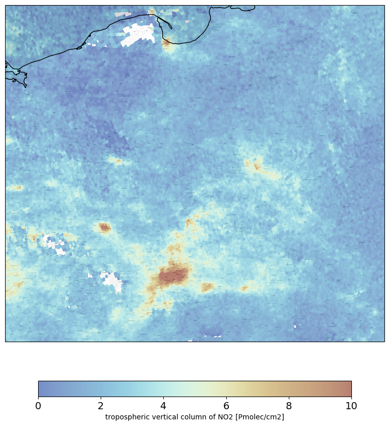
Eine Visualisierung erstellen

boundaries=[14, 25, 49, 55.0]                       #define boundaries (W, E, S, N)

fig = plt.figure(figsize=(10,10))                   #size of the figure
bmap=cimgt.Stamen(style='toner-lite')               #set background
ax = plt.axes(projection=bmap.crs)
ax.set_extent(boundaries,crs = ccrs.PlateCarree())

zoom = 10
ax.add_image(bmap, zoom)

img = plt.pcolormesh(gridlon, gridlat,
                     no2[0,:,:], vmin=vmin, vmax=vmax,
                     cmap=colortable,
                     transform=ccrs.PlateCarree(),alpha = 0.55)
ax.coastlines()

cbar = fig.colorbar(img, ax=ax,orientation='horizontal', fraction=0.04, pad=0.1)
cbar.set_label(f'{no2_description} [{no2_units}]')
cbar.ax.tick_params(labelsize=14)

plt.show()

TEIL #2 - Umrechnung und zonale Statistiken

Hier wird gezeigt, wie Sentinel-5P netCDF Daten in GeoTiff Format umgewandelt werden und zonale Statistiken mit CREODIAS berechnet werden

In diesem Teil decken wir folgendes ab:

netCDF in GeoTiff konvertieren

Berechnung der mittleren troposphärischen NO2-Säule (NO2 TVCD) für jeden polnischen Bezirk und Speichern der Ergebnisse als neu erstellte Shape-Datei

Plotten der netCDF - NO2 TVCD-Werte für das Gebiet von Interesse

Darstellung der mittleren NO2 TVCD-Werte für jeden polnischen Bezirk als thematische Karte

Exportieren der neu erstellten Karte in ein .jpg-Format

Mittlere NO2 TVCD-Werte für jeden polnischen Bezirk in einen Datenrahmen einfügen und als .csv exportieren

Datensätze, die verwendet werden sollen:

mean_no2_2023_03.nc - netCDF erstellt vom HARP-Prozessor

Bezirke in Polen https://www.geoportal.gov.pl/dane/panstwowy-rejestr-granic

Import libraries
#Import libraries

import pandas as pd
import geopandas as gpd
import xarray as xr
import numpy as np
import os
import matplotlib.pyplot as plt
from mpl_toolkits.basemap import Basemap
import rasterstats
import rasterio
import rioxarray
from rasterio.plot import show
from rasterio.transform import from_origin

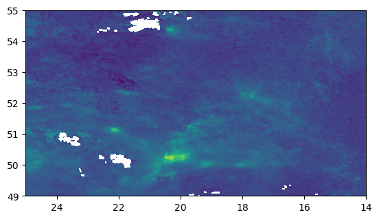
Bild als GeoTiff exportieren und Ergebnisse anzeigen

#open the netcdf file
r1 = xr.open_dataset('mean_no2_2023_03.nc')

#extract the tropospheric_NO2_column_number_density variable
no2 = r1['tropospheric_NO2_column_number_density'].values[0,:,:]
#reverse order of the values within the array
no2 = no2[::-1]

#get the latitude and longitude coordinates
y = r1['latitude'].values
x = r1['longitude'].values

#reverse the latitude and longitude coordinates
y = y[::-1]
x = x[::-1]

#convert the DataArray to a rioxarray DataArray
da = xr.DataArray(no2,
                  coords={'y': y, 'x': x},
                  dims=('y', 'x'),
                  attrs={'crs': 'EPSG:4326'})

#save the rioxarray DataArray to a GeoTIFF file with CRS 4326
da.rio.to_raster('mean_no2_2023_03.tif', crs='EPSG:4326')

#open new-crtead raster
src = rasterio.open("mean_no2_2023_03.tif")

#plot the new-created raster
show(src)

Berechnung der mittleren NO2 TVCD für jeden polnischen Bezirk und Speicherung der Ergebnisse als neu erstelltes Shapefile

# -*- coding: utf-8 -*-
#read shapefile of districts in Poland
shapefile_path = 'poland_pow.shp'
poland_pow = gpd.read_file(shapefile_path)

#define the affine transformation (pixel size and coordinates of the top-left corner of the raster)
affine = rasterio.transform.from_bounds(min(x), min(y),
                                        max(x), max(y),
                                        len(da.x), len(da.y))

#loop over the polygons in the poland_pow GeoDataFrame and calculate the mean NO2 TVCD for each polygon
mean_no2 = []
for i, row in poland_pow.iterrows():
    #extract the geometry of the polygon
    geometry = row.geometry
    #calculate the mean NO2 TVCD for the polygon
    mean_no2p = rasterstats.zonal_stats(geometry,
                                        da.values,
                                        affine=affine,
                                        nodata=-999,
                                        stats=['mean'],
                                        nan='ignore')[0]['mean']
    #add the mean NO2 TVCD value to the poland_pow GeoDataFrame properties
    poland_pow.loc[i, 'mean_no2'] = mean_no2p

#encode names of districts to UTF-8
poland_pow['JPT_NAZWA_'] = poland_pow['JPT_NAZWA_'].apply(lambda x: x.encode('latin-1').decode('utf-8'))
#save the GeoDataFrame with the mean NO2 TVCD values to a new shapefile
poland_pow.to_file('nuts_2023_03.shp', encoding='utf-8')

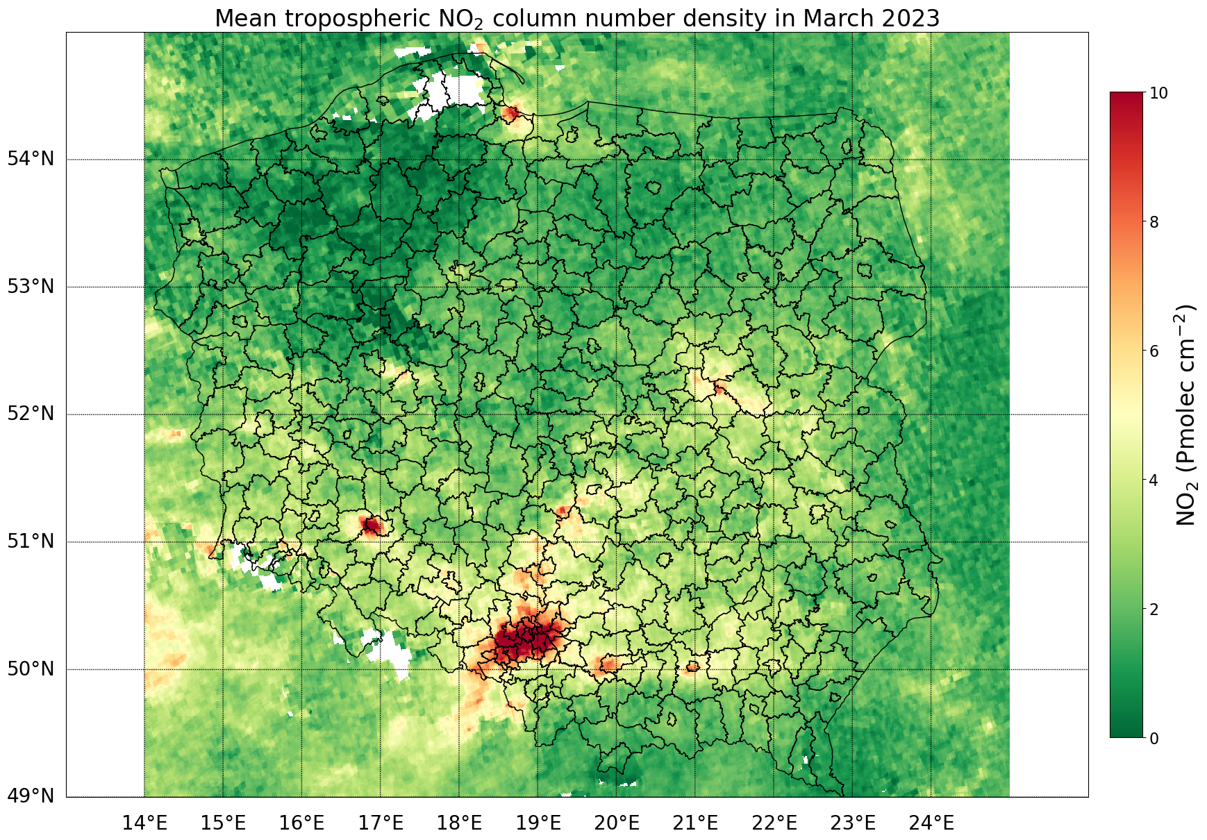
Plotten der netCDF - NO2 TVCD Werte für das Gebiet von Interesse - Polen

#open the netCDF file
nc_file = xr.open_dataset('mean_no2_2023_03.nc')

#read the tropospheric_NO2_column_number_density variable
no2_tvcd = nc_file['tropospheric_NO2_column_number_density'].values[0,:,]

#get the latitude and longitude coordinates from nc_file
lat = nc_file['latitude'].values
lon = nc_file['longitude'].values

#create the figure and Basemap instance
fig = plt.figure(figsize=(20,20))

#create a basemap with the desired projection and latitude/longitude bounds - Poland
m = Basemap(projection='cyl', llcrnrlat=49, urcrnrlat=55,
            llcrnrlon=13, urcrnrlon=26, resolution='c')

#plot NO2 TVCD on basemap
x, y = m(lon, lat)
m.pcolormesh(x, y, no2_tvcd, cmap='RdYlGn_r', vmin=0, vmax=10)

#add coordinates grid
m.drawparallels(np.arange(49, 55, 1), labels=[1,0,0,0], fontsize=20)
m.drawmeridians(np.arange(14, 25, 1), labels=[0,0,0,1], fontsize=20)

#read shapefile of districts in Poland
shapefile_path = 'poland_pow.shp'               #define path
poland_nuts = gpd.read_file(shapefile_path)     #read file containing districts of Poland

#plot districts on map
poland_nuts.plot(ax=plt.gca(), facecolor='none', edgecolor='black', linewidth=1)

#add colorbar
cbar = plt.colorbar(fraction=0.03, pad=0.02)
cbar.ax.set_ylabel('NO$_2$ (Pmolec cm$^{-2}$)', fontsize=24)
cbar.ax.tick_params(labelsize=16)

#plot title
plt.title('Mean tropospheric NO$_2$ column number density in March 2023', fontsize=24)

#show plot
plt.show()

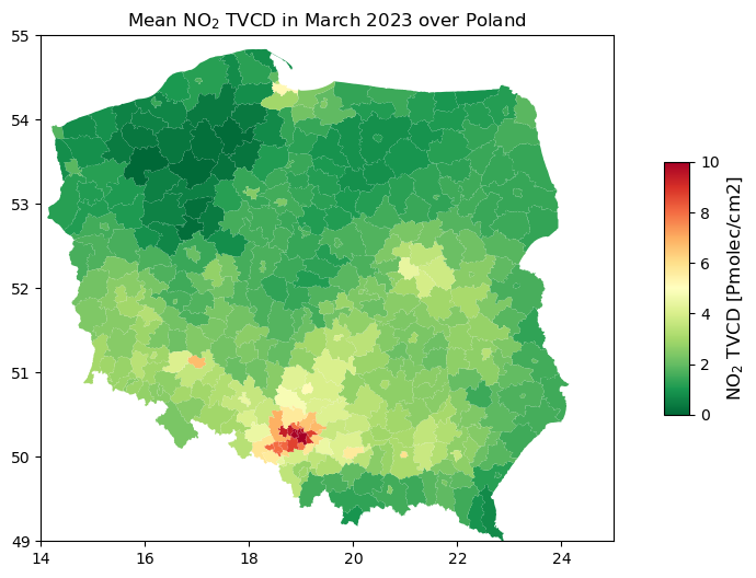
Darstellung der mittleren NO2 TVCD für jeden polnischen Bezirk - Erstellung einer thematischen Karte

#read shapefile of NUTS3 regions in Poland
shapefile_path = 'nuts_2023_03.shp'          #define path
poland_nuts = gpd.read_file(shapefile_path)  #read file containing districts of Poland

#create a figure
fig, ax1 = plt.subplots(ncols=1, figsize=(12, 6))

#plot choropleth based on mean NO2 TVCD iver Poland
poland_nuts.plot(column='mean_no2',                  #mean_no2 is a column contains mean NO2 TVCD for each polygon
                 cmap='RdYlGn_r', ax=ax1)            #cmap - color ramp from green to red
ax1.set_xlim(14, 25)                                 #W-E extent of Poland
ax1.set_ylim(49, 55)                                 #S-N extent of Poland
ax1.set_title('Mean NO$_2$ TVCD in March 2023 over Poland')    #title of plot

#add a colorbar reffering to the the NO2 TVCD
vmin, vmax = [0, 10]                           #min and max value on colorbar
cbar = plt.cm.ScalarMappable(cmap='RdYlGn_r', norm=plt.Normalize(vmin=vmin, vmax=vmax))
plt.colorbar(cbar, ax=ax1, shrink=0.5, aspect=10).set_label('NO$_2$ TVCD [Pmolec/cm2]', fontsize=12)

#show the plot
plt.show()

Exportieren Sie ein Bild der mittleren NO2 TVCD für jeden polnischen Bezirk in ein .jpg-Format

#save a plot as a .jpg
fig.savefig('POLAND_NO2_2023_03.jpg', dpi=300)

Fügen Sie die mittleren NO2 TVCD für jeden polnischen Bezirk in einen Pandas DataFrame ein

#get the mean NO2 TVCD values for each polygon in the Poland shapefile and round to two decimal places
no2_means = round(poland_nuts['mean_no2'],2)

#create a Pandas DataFrame with the mean NO2 TVCD values and their corresponding polygon names
NO2_df = pd.DataFrame({'Polygon': poland_nuts['JPT_NAZWA_'], 'Mean NO2': no2_means})

#sort the Poland's districts in descending order by the mean NO2 values values
NO2_df = NO2_df.sort_values(by='Mean NO2', ascending=False)

#print the DataFrame
print(NO2_df)

                         Polygon  Mean NO2
            powiat Katowice     10.76
         powiat Ruda Śląska     10.70
      powiat Świętochłowice     10.66
             powiat Chorzów     10.64
 powiat Siemianowice Śląskie     10.29
..                           ...       ...

225 powiat chodzieski 0.52 19 powiat obornicki 0.51 329 powiat chojnicki 0.48 174 powiat złotowski 0.42 328 powiat drawski 0.36

[380 rows x 2 columns]

Export der mittleren NO2 TVCD für jeden polnischen Bezirk in eine .csv-Datei

NO2_df.to_csv('NO2_df.csv')